Meta-analysis
Charles Martin
December 2019
- Basic principle
- Selecting studies
- Effect size
- Visualization
- The publication bias
- Random effects models?
- References
library(dplyr) # data manipulation
library(ggplot2) # visualizations
library(metafor) # ready-made meta-analysis code
library(gt) # nice tables
Basic principle
Scientific question
Does playing Mozart to newborns improves their IQ?
You look a bit around and find 3 studies :
etudes <- data.frame(
  article = c("A","B","C"),
  y = c(0.5, 0.01, -0.1), # 0 no effect, <0 negative effect, >0 positive effect
  n = c(10,150,12),
  v = c(0.04,0.01, 0.03) # variance
)
etudes %>% gt
| article | y | n | v |
|---|---|---|---|
| A | 0.50 | 10 | 0.04 |
| B | 0.01 | 150 | 0.01 |
| C | -0.10 | 12 | 0.03 |
A simplistic way
etudes %>%
  summarise(
    effet_resume = mean(y)
  )
  effet_resume
1    0.1366667
Weighted mean
When we talk about mean, we usually refer to the arithmetic mean :
(1 + 2 + 3 + 4) / 4
[1] 2.5
Implicitly, we give an equal weight to all items :
(1*1 + 1*2 + 1*3 + 1*4) / (1 + 1 + 1 + 1)
[1] 2.5
But we could also have given more weight to some items, for example giving more weight to more recent entries
(0.125*1 + 0.25*2 + 0.5*3 + 1*4) / (0.125 + 0.25 + 0.5 + 1)
[1] 3.266667
There’s an R function that does this for us :
weighted.mean(
  c(1,2,3,4),
  c(0.125,0.25,0.5,1)
)
[1] 3.266667
A meta-analysis is a weighted mean
The most precise studies will have more weight in our calculation of the average effect.
One classical way to do this is to use the inverse of variance as weights.
IMPORTANT CAVEAT : there are two definitions of variance
The classical definition is usually defined on a sample as :
v = sum( (x-mean(x))^2 / (length(x)-1) )
From which we can calculate the standard deviation of our sample : : sd = sqrt(v).
Both these measures are of descriptive nature.
You also probably remember that, to go from the standard deviation of a sample to the standard error of a parameter (i.e. the error around its estimate), we use the formula :
se = sd / sqrt(n)
On the other hand, in the Borenstein book (see refs at bottom), when they talk about variance, they (implicitly) talk about the variance of the error around a parameter (sampling variance), which is :
v = se^2
Calculation examples
Knowing the above, we can now calculate our first meta-analysis :
etudes %>%
  summarise(
    effet_pondere = weighted.mean(y,1/v)
  )
  effet_pondere
1    0.06421053
With the metafor package, we arrive to the exact same number :
m <- rma(
  yi = y,
  vi = v,
  data = etudes,
  method = "FE"
)
m
Fixed-Effects Model (k = 3)

Test for Heterogeneity:
Q(df = 2) = 5.9405, p-val = 0.0513

Model Results:

estimate      se    zval    pval    ci.lb   ci.ub
  0.0642  0.0795  0.8080  0.4191  -0.0916  0.2200

---
Signif. codes:  0 '***' 0.001 '**' 0.01 '*' 0.05 '.' 0.1 ' ' 1
This function also gives the the confidence interval around our mean value (and some other things we’ll look into later).
In this case, the 95% confidence interval of our summary effect does not exclude zero, so there is not significant effect to play Mozart to newborns.
Selecting studies
It is always a good idea to search for studies in a reproducible way, e.g. by searching on the Scopus database
(https://www2.scopus.com/search/form.uri?display=basic):
TITLE-ABS-KEY ( music AND ( baby OR toddler OR newborn ) AND ( iq OR intelligence ) )
Then you can export that list of studies to freeze your search.
It is often recommended to scan the references from each these articles to make sure you have not missed anything.
Also, keep a detailed trace of all the dataset building and filtering steps. You’ll need to cite these steps with their associated numbers when writing your manuscript. E.g. :
- # of studies found in the Scopus search
- # of studies found from references
- # of duplicate studies eliminated
- # of studies eliminated by reading the abstract
- # of studies eliminated for other criteria (wrong taxonomic group, lacking necessary data, etc.)
- # of studies included in the meta-analysis
Effect size
The issue
It is unlikely that all the studies you’ve found measured the target effect in exactly the same way.
In our example, we could for example find :
- a correlation between the number of music hours per week and IQ
- a T test between groups with and without music
- a slope between the number of songs played daily and IQ
- a slope between the number of classic music albums owned by the parents and IQ
Correlations are scale independent, but for the other measurements, the numbers found are highly dependent on the scale of the X variable, and will need to be standardized for comparison purposes.
Standardizing effect sizes
There are dozens of ways to standardize effect sizes, depending on the nature of the data at hand (mean differences, slopes, proportions, etc.)
In all cases, the idea is to find a measure that can remove scale differences.
E.g. for mean differences, one often uses Cohen’s d. Its calculate looks a lot like the calculation for a t statistic :
d = (x1 - x2) / S_within
A variance (sensu Borenstein et al. 2011) formula is also associated with each of these standardized effect sizes.
V_d = (n1 + n2 / n1*n2) + (d^2 / 2*(n1+n2))
It can also happen that some measures, although on a standardized scale, also need to be converted because their distributional properties are not appropriate for meta-analysis calculations. E.g. Pearson’s r must be converted into Fisher’s z because r’s variance is not homogenous across the spectrum of values.
z = 0.5 * log((1+r)/(1-r))
V_z = 1/(n-3)
Automation
The metafor package includes a function which can facilitate effect size calculations. It is nevertheless limited to one type of conversion per call (e.g. from correlation to Fisher’s z) :
etudes2 <- data.frame(
  etude = c("A","B"),
  r = c(0.6, -0.2),
  n = c(32,16)
)
escalc(
  measure = "ZCOR",
  ri = r,
  ni = n,
  data = etudes2
) %>%
  gt
| etude | r | n | yi | vi |
|---|---|---|---|---|
| A | 0.6 | 32 | 0.6931472 | 0.03448276 |
| B | -0.2 | 16 | -0.2027326 | 0.07692308 |
Uniformization
One of the issue you’ll often face is that you’ll find many different measurement types (correlations, mean differences, etc.) and that each of these will convert to a different standardize effect size. You’ll often come to a point where you have Cohen’s ds, Fisher’s zs and Hedge’s g to analyze together.
There is a whole chapter in the Borenstein book dedicated solely to the conversions between effect sizes. You just need to patiently look them up.
Classic ecological issues
In ecology, you’ll often be studying phenomenons that are described by slopes. These slopes will need to be manually converted to be included in the meta-analysis, and this conversion is not necessarily simple.
If you have access to the raw that, know that the formula to calculate a regression slope is :
slope = r*(Sy / Sx)
you can convert a slope to a correlation by dividing it by the Sy/Sx ratio.
Otherwise, if you don’t have access to standard deviations, it is also possible to calculate standardized from t values and df. Equations are in a hard to read paper from 1982 (Friedman, Simplified determination of statistical power, magnitude of effect and research sample sizes. Educ Psychol Meas 42:521–526).
For our example
The data used in our study were already in a standardized effect size : the log-response ratio.
I.e. the log of the ratio between with and without music responses
Without the log transformation, our numbers would have looked like :
etudes %>%
  mutate(R = exp(y)) %>%
  gt
| article | y | n | v | R |
|---|---|---|---|---|
| A | 0.50 | 10 | 0.04 | 1.6487213 |
| B | 0.01 | 150 | 0.01 | 1.0100502 |
| C | -0.10 | 12 | 0.03 | 0.9048374 |
Which can be read as : 64% increase, 1% increase and 10% decrease of IQ.
Such ratios, although easy to understand, become a problem once entered into a model because of asymmetries. When the denominator of the ratio is larger, the ratio can take almost any value and get into real large numbers, although if the denominator of the ratio is smaller, the ratio is “stuck” between 0 and 1 :
1/100 # 0.99 under 1
[1] 0.01
100/1 # 99 above 1
[1] 100
Le log transformation can re-establish this symmetry
log(1/100) # 4.6 below zero
[1] -4.60517
log(100/1) # 4.6 above zero
[1] 4.60517
Visualization
The classical way to visualize a meta-analysis is with what is called a forest plot :
forest(m, order = "obs", slab = etudes$article)
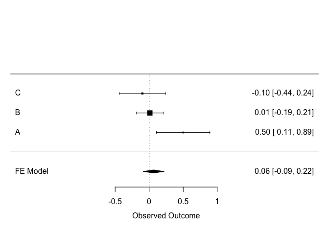
Each line from the plot is a study. The effect size measured in each study is displayed, along with its confidence interval. The size of the square corresponds to the weight of the study in the calculation.
The last line is the summarized effect, as calculated above.
Sometimes it can be helpful to back-transform the standardized effect size to a version easier to interpret :
exp(-0.09)
[1] 0.9139312
exp(0.22)
[1] 1.246077
So, the summarized effect size is somewhere between a 25% increase and a 9% decrease in IQ
The publication bias
One issue that needs to be addressed when doing a meta-analysis is that it could happen that results that did not fit the expected results were simply not published.
Visualization
One way to visualize this issue is with a funnel plot.
funnel(m)
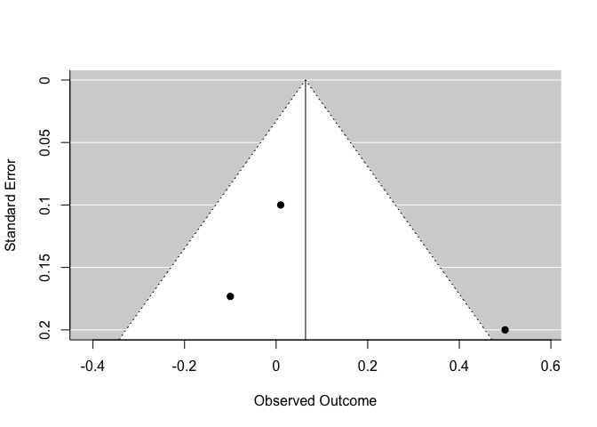
On the y axis, you have the precision of each study and on the x axis, the effect size reported. Normally, the more precise a study is, the closer it should be to the synthesized effect. At the bottom of the funnel, the less precise studies should vary more around the mean.
You need to be particularly wary of publication bias if points in this plot are strongly asymmetrical.
Statistical tests
regtest(m, model = "lm", predictor = "sei")
Regression Test for Funnel Plot Asymmetry

model:     weighted regression with multiplicative dispersion
predictor: standard error

test for funnel plot asymmetry: t = 0.6405, df = 1, p = 0.6373
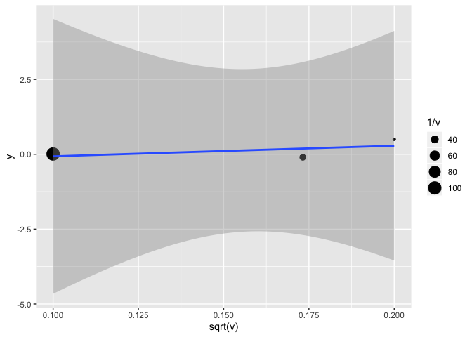
The classic Egger test, in short, is a regression of the estimate on the standard error.
(lm(y~sqrt(v), weights = 1/v, data = etudes))
etudes %>%
  ggplot(aes(x = sqrt(v), y = y)) +
  geom_point(aes(size = 1/v)) +
  geom_smooth(method = "lm") # attention, il faudrait aussi ajuster le poids de chaque observation à 1/v
There are other ways to test for publication bias, for example with sensitivity analyses.
One of these methods is the Trim & Fill procure. An algorithm estimates how many studies are missing on one side of the analysis, and then recalculates our summarized effect by adding ghost studies. This new estimate must not be interpreted as a more valid result. It must only be used to evaluate the sensitivity of our results.
(in this example, we are using another dataset because there are not missing studies in our example)
res <- rma(yi, vi, data = dat.hackshaw1998)
taf <- trimfill(res)
funnel(taf)
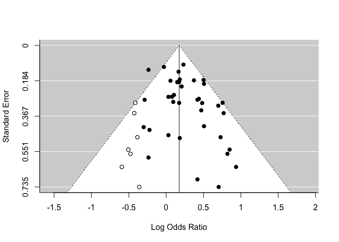
taf
Estimated number of missing studies on the left side: 7 (SE = 4.0399)

Random-Effects Model (k = 44; tau^2 estimator: REML)

tau^2 (estimated amount of total heterogeneity): 0.0245 (SE = 0.0183)
tau (square root of estimated tau^2 value):      0.1565
I^2 (total heterogeneity / total variability):   28.86%
H^2 (total variability / sampling variability):  1.41

Test for Heterogeneity:
Q(df = 43) = 60.5196, p-val = 0.0400

Model Results:

estimate      se    zval    pval   ci.lb   ci.ub
  0.1745  0.0484  3.6015  0.0003  0.0795  0.2694  ***

---
Signif. codes:  0 '***' 0.001 '**' 0.01 '*' 0.05 '.' 0.1 ' ' 1
Random effects models?
Up until now, we have described a simple meta-analysis model, where we assumed that, in the absence of measurement noise, all studies would have given exactly the same result.
It is possible (and almost always the case in ecology), that the effect size depends on the context in which the study was performed or on the group of individuals selected.
In our Mozart example, one could easily imagine that the effect of classic music might be context sensitive, depending on the cultural context.
If it is the case, we are not looking for an absolute and identical effect size anymore. We assume that there exists a population of possible effect sizes, which depend on measurement the context. The error (or noise) on our effect size then has two sources : the internal error in each study, and the between study variability. In this case, we need to apply a random effects model.
Implications
The random effects model adds an additional variance component, which must also be estimated. Model calculations are then more complex and must use maximum likelihood methods, instead of ordinary least squares in the fixed effects model.
The important thing to consider is that, the weight given to each study will be calculated differently in random effects models. Since our model must be representative of the between-study variability, it must be more balanced in its calculation. Even if a study is very imprecise, the information it brings about between-study variability must still be accounted for (and vice versa, a highly precise study will have a lower weight, because it must not completely erase the between-study differences)
Calculations
In the metafor package, random effects models are adjusted with the same function as fixed effects, only removing the method = 'FE' argument.
m2 <- rma(
  yi = y,
  vi = v,
  data = etudes
)
m2
Random-Effects Model (k = 3; tau^2 estimator: REML)

tau^2 (estimated amount of total heterogeneity): 0.0574 (SE = 0.0827)
tau (square root of estimated tau^2 value):      0.2397
I^2 (total heterogeneity / total variability):   70.75%
H^2 (total variability / sampling variability):  3.42

Test for Heterogeneity:
Q(df = 2) = 5.9405, p-val = 0.0513

Model Results:

estimate      se    zval    pval    ci.lb   ci.ub
  0.1132  0.1655  0.6843  0.4938  -0.2111  0.4375

---
Signif. codes:  0 '***' 0.001 '**' 0.01 '*' 0.05 '.' 0.1 ' ' 1
This result is very close to the original one, but more conservative. I.e. it is less influenced by the highly precise study.
The results output now contains additional information. Tau^2 is the between-study variance. I^2 is the proportion of the total variance that comes from the between-study heterogeneity. The higher this number, the more different the studies are from one another.
The output also contains a test for heterogeneity, which determines if the between-study heterogeneity is statistically significant or now. Although intuitively one could use this value to determine if we need a random effects model or not, most authors recommend that, if you have theoretical reasons to use a random effects model, just apply that model, disregarding the results from this test.
References
Borenstein, M., Hedges, L. V., Higgins, J. P., & Rothstein, H. R. (2011). Introduction to meta-analysis. John Wiley & Sons.
Viechtbauer, W. (2010). Conducting meta-analyses in R with the metafor package. Journal of Statistical Software, 36(3), 1-48. URL: http://www.jstatsoft.org/v36/i03/
Viechtbauer, W. (2021). The metafor Package: A Meta-Analysis Package for R. https://www.metafor-project.org/doku.php/metafor